44 chart data labels excel
Change the format of data labels in a chart To get there, after adding your data labels, select the data label to format, and then click Chart Elements > Data Labels > More Options. To go to the appropriate area, click one of the four icons ( Fill & Line, Effects, Size & Properties ( Layout & Properties in Outlook or Word), or Label Options) shown here. DataLabels object (Excel) | Microsoft Learn The following example sets the number format for data labels on series one on chart sheet one. With Charts(1).SeriesCollection(1) .HasDataLabels = True .DataLabels.NumberFormat = "##.##" End With Use DataLabels (index), where index is the data-label index number, to return a single DataLabel object. The following example sets the number format ...
Present data in a chart - support.microsoft.com Chart created from worksheet data. Excel supports many types of charts to help you display data in ways that are meaningful to your audience. When you create a chart or change an existing chart, you can select from a variety of chart types (such as a column chart or a pie chart) and their subtypes (such as a stacked column chart or a pie in 3-D ...

Chart data labels excel
Edit titles or data labels in a chart - support.microsoft.com On a chart, click one time or two times on the data label that you want to link to a corresponding worksheet cell. The first click selects the data labels for the whole data series, and the second click selects the individual data label. Right-click the data label, and then click Format Data Label or Format Data Labels. Example: Charts with Data Labels — XlsxWriter Documentation Chart 1 in the following example is a chart with standard data labels: Chart 6 is a chart with custom data labels referenced from worksheet cells: Chart 7 is a chart with a mix of custom and default labels. The None items will get the default value. We also set a font for the custom items as an extra example: Chart 8 is a chart with some ... Labels in a Scatter Chart - Microsoft Community I have a scatter chart with data points in the chart. The data points have lables. In addtion to these labels, I would like to place my cursor on a particular data point and it would show the contents of a particular cell. This would be addtional information about the data point but only shown when I place my cursor over it. This is is in ...
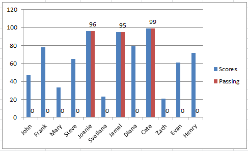
Chart data labels excel. How to hide zero data labels in chart in Excel? - ExtendOffice If you want to hide zero data labels in chart, please do as follow: 1. Right click at one of the data labels, and select Format Data Labels from the context menu. See screenshot: 2. In the Format Data Labels dialog, Click Number in left pane, then select Custom from the Category list box, and type #"" into the Format Code text box, and click Add button to add it to Type list box. › examples › pie-chartCreate a Pie Chart in Excel (In Easy Steps) - Excel Easy 6. Create the pie chart (repeat steps 2-3). 7. Click the legend at the bottom and press Delete. 8. Select the pie chart. 9. Click the + button on the right side of the chart and click the check box next to Data Labels. 10. Click the paintbrush icon on the right side of the chart and change the color scheme of the pie chart. Result: 11. How to Use Cell Values for Excel Chart Labels - How-To Geek Select the chart, choose the "Chart Elements" option, click the "Data Labels" arrow, and then "More Options." Uncheck the "Value" box and check the "Value From Cells" box. Select cells C2:C6 to use for the data label range and then click the "OK" button. The values from these cells are now used for the chart data labels. Excel: How to Create a Bubble Chart with Labels - Statology Step 3: Add Labels. To add labels to the bubble chart, click anywhere on the chart and then click the green plus "+" sign in the top right corner. Then click the arrow next to Data Labels and then click More Options in the dropdown menu: In the panel that appears on the right side of the screen, check the box next to Value From Cells within ...
How to Add Data Labels in Excel - Excelchat | Excelchat After inserting a chart in Excel 2010 and earlier versions we need to do the followings to add data labels to the chart; Click inside the chart area to display the Chart Tools. Figure 2. Chart Tools Click on Layout tab of the Chart Tools. In Labels group, click on Data Labels and select the position to add labels to the chart. Figure 3. chandoo.org › wp › change-data-labels-in-chartsHow to Change Excel Chart Data Labels to Custom Values? May 05, 2010 · Now, click on any data label. This will select “all” data labels. Now click once again. At this point excel will select only one data label. Go to Formula bar, press = and point to the cell where the data label for that chart data point is defined. Repeat the process for all other data labels, one after another. See the screencast. › how-to-create-excel-pie-chartsHow to Make a Pie Chart in Excel & Add Rich Data Labels to ... Sep 08, 2022 · In this article, we are going to see a detailed description of how to make a pie chart in excel. One can easily create a pie chart and add rich data labels, to one’s pie chart in Excel. So, let’s see how to effectively use a pie chart and add rich data labels to your chart, in order to present data, using a simple tennis related example. support.microsoft.com › en-us › officePresent data in a chart - support.microsoft.com Add titles and data labels to a chart To help clarify the information that appears in your chart, you can add a chart title, axis titles, and data labels. Add a legend or data table You can show or hide a legend, change its location, or modify the legend entries.
Add or remove data labels in a chart - support.microsoft.com Click the data series or chart. To label one data point, after clicking the series, click that data point. In the upper right corner, next to the chart, click Add Chart Element > Data Labels. To change the location, click the arrow, and choose an option. If you want to show your data label inside a text bubble shape, click Data Callout. Format Data Labels in Excel- Instructions - TeachUcomp, Inc. Nov 14, 2019 · Alternatively, you can right-click the desired set of data labels to format within the chart. Then select the “Format Data Labels…” command from the pop-up menu that appears to format data labels in Excel. Using either method then displays the “Format Data Labels” task pane at the right side of the screen. Format Data Labels in Excel ... How to add total labels to stacked column chart in Excel? - ExtendOffice 1. Create the stacked column chart. Select the source data, and click Insert > Insert Column or Bar Chart > Stacked Column. 2. Select the stacked column chart, and click Kutools > Charts > Chart Tools > Add Sum Labels to Chart. Then all total labels are added to every data point in the stacked column chart immediately. Create a Pie Chart in Excel (In Easy Steps) - Excel Easy 6. Create the pie chart (repeat steps 2-3). 7. Click the legend at the bottom and press Delete. 8. Select the pie chart. 9. Click the + button on the right side of the chart and click the check box next to Data Labels. 10. Click the paintbrush icon on the right side of the chart and change the color scheme of the pie chart. Result: 11.
Microsoft Excel Tutorials: Add Data Labels to a Pie Chart
How to Add Data Labels to Scatter Plot in Excel (2 Easy Ways) - ExcelDemy 2 Methods to Add Data Labels to Scatter Plot in Excel 1. Using Chart Elements Options to Add Data Labels to Scatter Chart in Excel 2. Applying VBA Code to Add Data Labels to Scatter Plot in Excel How to Remove Data Labels 1. Using Add Chart Element 2. Pressing the Delete Key 3. Utilizing the Delete Option Conclusion Related Articles

How to fix wrapped data labels in a pie chart | Sage Intelligence
Excel charts: add title, customize chart axis, legend and data labels Click the Chart Elements button, and select the Data Labels option. For example, this is how we can add labels to one of the data series in our Excel chart: For specific chart types, such as pie chart, you can also choose the labels location. For this, click the arrow next to Data Labels, and choose the option you want.

Change Chart Data Labels : Chart Data « Chart « Microsoft ...
How to Make a Pie Chart in Excel & Add Rich Data Labels to The Chart! Sep 08, 2022 · A pie chart is used to showcase parts of a whole or the proportions of a whole. There should be about five pieces in a pie chart if there are too many slices, then it’s best to use another type of chart or a pie of pie chart in order to showcase the data better. In this article, we are going to see a detailed description of how to make a pie chart in excel.
How to Add Data Labels to your Excel Chart in Excel 2013
How to insert or add axis labels in Excel 365 charts (with Example)? Adding axis title labels to Excel chart. Thanks for the question let's break down the process into simple steps. We'll use a simple example of creating an XY chart, but the process is similar for every graph you might be plotting in Excel. In Microsoft Excel, select your data and hit Insert, then from the Ribbon pick the scatter chart.

Two-Level Axis Labels (Microsoft Excel)
depictdatastudio.com › how-to-make-a-side-by-sideHow to Make a Side by Side Bar Chart in Excel | Depict Data ... Jun 10, 2013 · Step 6: Populate the second chart with Coalition B’s data. Use the “select data” feature to put Coalition B’s percentages into the chart. Step 7: Adjust the second chart’s bar color and title. Step 8: Delete the second chart’s axis labels. Yep, you’re right, the second chart’s bars are going to get waaaaaay too long.

How to Customize Your Excel Pivot Chart Data Labels - dummies
How to add data labels from different column in an Excel chart? This method will guide you to manually add a data label from a cell of different column at a time in an Excel chart. 1.Right click the data series in the chart, and select Add Data Labels > Add Data Labels from the context menu to add data labels.. 2.

Custom Data Labels with Colors and Symbols in Excel Charts ...
How to add or move data labels in Excel chart? - ExtendOffice In Excel 2013 or 2016. 1. Click the chart to show the Chart Elements button . 2. Then click the Chart Elements, and check Data Labels, then you can click the arrow to choose an option about the data labels in the sub menu. See screenshot: In Excel 2010 or 2007. 1. click on the chart to show the Layout tab in the Chart Tools group. See ...

Custom data labels in a chart
How to Change Excel Chart Data Labels to Custom Values? - Chandoo.org May 05, 2010 · Now, click on any data label. This will select “all” data labels. Now click once again. At this point excel will select only one data label. Go to Formula bar, press = and point to the cell where the data label for that chart data point is defined. Repeat the process for all other data labels, one after another. See the screencast.
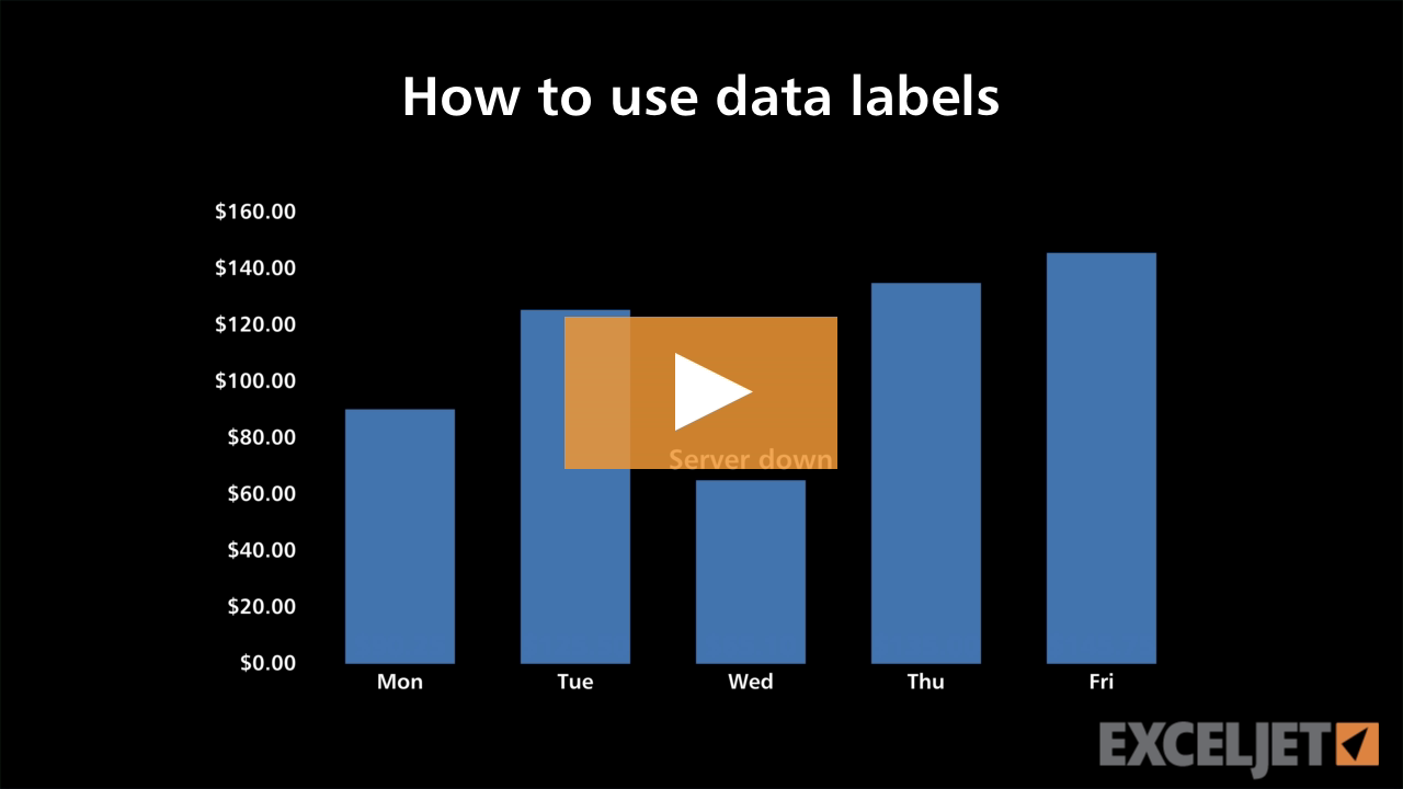
Excel tutorial: How to use data labels
How to create Custom Data Labels in Excel Charts - Efficiency 365 Create the chart as usual. Add default data labels. Click on each unwanted label (using slow double click) and delete it. Select each item where you want the custom label one at a time. Press F2 to move focus to the Formula editing box. Type the equal to sign. Now click on the cell which contains the appropriate label.

How to add data labels from different column in an Excel chart?
Add data labels excel - cgc.abedini.info Re: 2 data labels on a Waterfall Chart. Hello. I do have quite a similar question. I have a waterfall, but to analyze the data correclty I would always need to see the percentages as well (and how they changed vs the previous period). In best case like an additional line. But I am open for other solutions as well.

Add data labels to your Excel bubble charts | TechRepublic
Edit titles or data labels in a chart - support.microsoft.com You can also place data labels in a standard position relative to their data markers. Depending on the chart type, you can choose from a variety of positioning options. On a chart, do one of the following: To reposition all data labels for an entire data series, click a data label once to select the data series.
Solved: Data labels overlap with Bar chart area - Microsoft ...
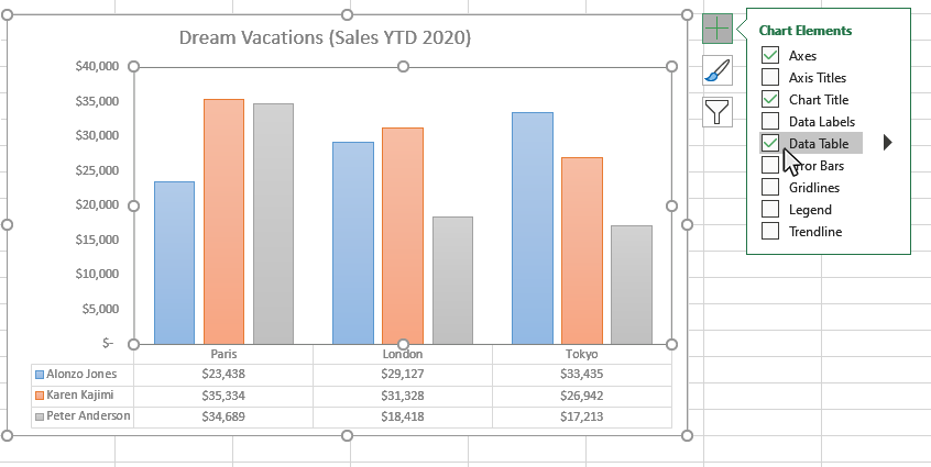
Add or remove data labels in a chart - support.microsoft.com Data labels make a chart easier to understand because they show details about a data series or its individual data points. For example, in the pie chart below, without the data labels it would be difficult to tell that coffee was 38% of total sales. ... You can add data labels to show the data point values from the Excel sheet in the chart ...

Quick Tip: Excel 2013 offers flexible data labels | TechRepublic
How to Create Charts in Excel (In Easy Steps) - Excel Easy 1. Select the chart. 2. Click the + button on the right side of the chart, click the arrow next to Legend and click Right. Result: Data Labels. You can use data labels to focus your readers' attention on a single data series or data point. 1. Select the chart. 2. Click a green bar to select the Jun data series. 3.

How to Add Two Data Labels in Excel Chart (with Easy Steps ...
How to add data labels from different column in an Excel chart? Right click the data series in the chart, and select Add Data Labels > Add Data Labels from the context menu to add data labels. 2. Click any data label to select all data labels, and then click the specified data label to select it only in the chart. 3.

Aligning data point labels inside bars | How-To | Data ...
support.microsoft.com › en-us › officeAdd or remove data labels in a chart - support.microsoft.com Click the data series or chart. To label one data point, after clicking the series, click that data point. In the upper right corner, next to the chart, click Add Chart Element > Data Labels. To change the location, click the arrow, and choose an option. If you want to show your data label inside a text bubble shape, click Data Callout.

How to Change Excel Chart Data Labels to Custom Values?
How to Insert Axis Labels In An Excel Chart | Excelchat The method below works in the same way in all versions of Excel. How to add horizontal axis labels in Excel 2016/2013 . We have a sample chart as shown below; Figure 2 – Adding Excel axis labels. Next, we will click on the chart to turn on the Chart Design tab; We will go to Chart Design and select Add Chart Element; Figure 3 – How to label ...

Excel charts: add title, customize chart axis, legend and ...
› format-data-labels-in-excelFormat Data Labels in Excel- Instructions - TeachUcomp, Inc. Nov 14, 2019 · Alternatively, you can right-click the desired set of data labels to format within the chart. Then select the “Format Data Labels…” command from the pop-up menu that appears to format data labels in Excel. Using either method then displays the “Format Data Labels” task pane at the right side of the screen. Format Data Labels in Excel ...
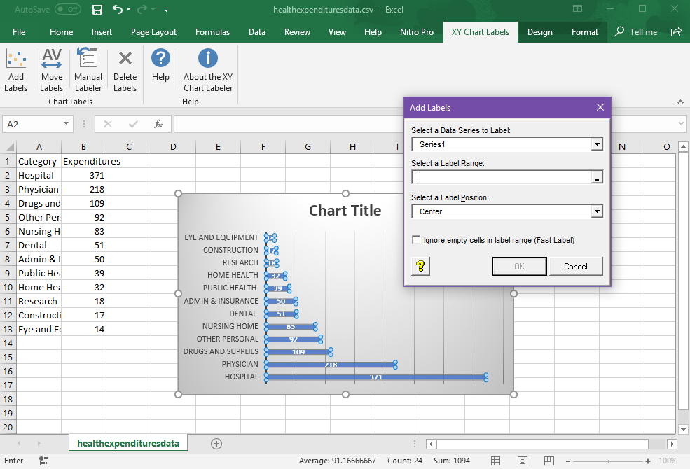
Add Labels to XY Chart Data Points in Excel with XY Chart Labeler
Data Labels in Excel Pivot Chart (Detailed Analysis) 7 Suitable Examples with Data Labels in Excel Pivot Chart Considering All Factors 1. Adding Data Labels in Pivot Chart 2. Set Cell Values as Data Labels 3. Showing Percentages as Data Labels 4. Changing Appearance of Pivot Chart Labels 5. Changing Background of Data Labels 6. Dynamic Pivot Chart Data Labels with Slicers 7.
Add Data Labels Outside End for Dynamic Label Threshold Chart ...
How to Make a Side by Side Bar Chart in Excel - Depict Data … Jun 10, 2013 · Step 6: Populate the second chart with Coalition B’s data. Use the “select data” feature to put Coalition B’s percentages into the chart. Step 7: Adjust the second chart’s bar color and title. Step 8: Delete the second chart’s axis labels. Yep, you’re right, the second chart’s bars are going to get waaaaaay too long.

Custom Excel Chart Label Positions • My Online Training Hub
How to Add Two Data Labels in Excel Chart (with Easy Steps) Select the data labels. Then right-click your mouse to bring the menu. Format Data Labels side-bar will appear. You will see many options available there. Check Category Name. Your chart will look like this. Now you can see the category and value in data labels. Read More: How to Format Data Labels in Excel (with Easy Steps) Things to Remember

Add or remove data labels in a chart
Chart.ApplyDataLabels method (Excel) | Microsoft Learn ApplyDataLabels ( Type, LegendKey, AutoText, HasLeaderLines, ShowSeriesName, ShowCategoryName, ShowValue, ShowPercentage, ShowBubbleSize, Separator) expression A variable that represents a Chart object. Parameters Example This example applies category labels to series one on Chart1. VB Charts ("Chart1").SeriesCollection (1).
Custom Chart Data Labels In Excel With Formulas
Labels in a Scatter Chart - Microsoft Community I have a scatter chart with data points in the chart. The data points have lables. In addtion to these labels, I would like to place my cursor on a particular data point and it would show the contents of a particular cell. This would be addtional information about the data point but only shown when I place my cursor over it. This is is in ...

Enable or Disable Excel Data Labels at the click of a button ...
Example: Charts with Data Labels — XlsxWriter Documentation Chart 1 in the following example is a chart with standard data labels: Chart 6 is a chart with custom data labels referenced from worksheet cells: Chart 7 is a chart with a mix of custom and default labels. The None items will get the default value. We also set a font for the custom items as an extra example: Chart 8 is a chart with some ...
Excel Data Labels: How to add totals as labels to a stacked ...
Edit titles or data labels in a chart - support.microsoft.com On a chart, click one time or two times on the data label that you want to link to a corresponding worksheet cell. The first click selects the data labels for the whole data series, and the second click selects the individual data label. Right-click the data label, and then click Format Data Label or Format Data Labels.

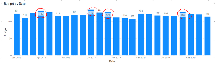
charts - Excel, giving data labels to only the top/bottom X ...

how to add data labels into Excel graphs — storytelling with data

Custom Excel Chart Label Positions • My Online Training Hub

Apply Custom Data Labels to Charted Points - Peltier Tech

Add or remove data labels in a chart
How to Add Data Tables to a Chart in Excel - Business ...
Solved: Area chart data labels not in correct positions ...
How to Place Labels Directly Through Your Line Graph in ...

How to add live total labels to graphs and charts in Excel ...
How to Place Labels Directly Through Your Line Graph in ...

Add data labels and callouts to charts in Excel 365 ...

Is it possible to conditionally format Data Labels on a ...

Custom Data Labels with Colors and Symbols in Excel Charts ...
/Capture-e92aa05671d543ceaf94080eb2687619.JPG)
Understanding Excel Chart Data Series, Data Points, and Data ...

Chart Data Labels in PowerPoint 2011 for Mac

Format Number Options for Chart Data Labels in Excel 2011 for Mac

Is there a way to add data labels as percentages on the ...

Adding Data Labels to Your Chart (Microsoft Excel)

Add or remove data labels in a chart

microsoft excel - Adding data label only to the last value ...
Post a Comment for "44 chart data labels excel"