41 excel chart add labels to data points
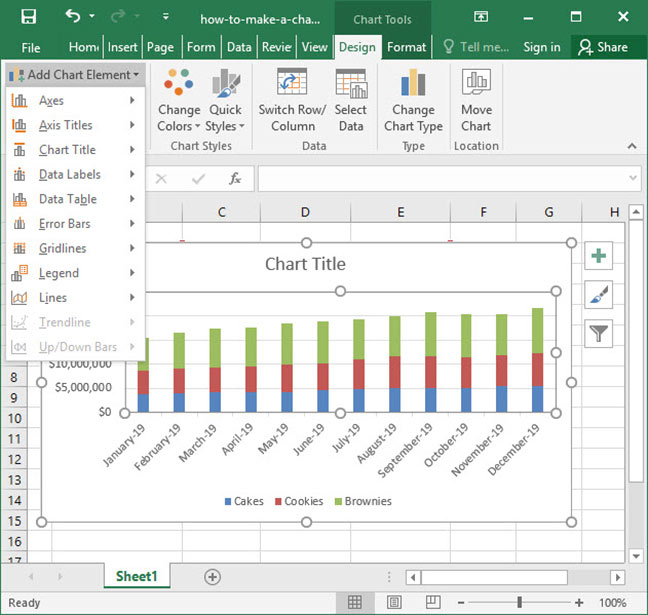
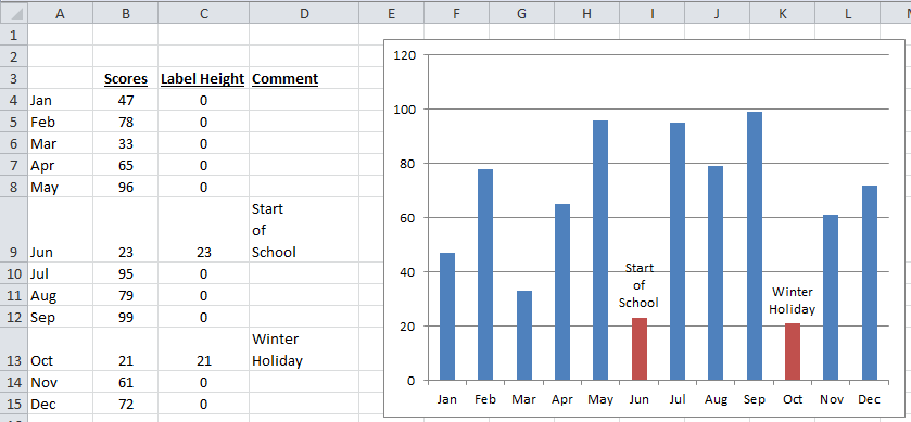
How to Create a Bar Chart in Excel with Multiple Bars? To fine tune the bar chart in excel, you can add a title to the graph. You can also add data labels. To add data labels, go to the Chart Design ribbon, and from the Add Chart Element, options select Add Data Labels. Adding data labels will add an extra flair to your graph. You can compare the score more easily and come to a conclusion faster. Modifying Axis Scale Labels (Microsoft Excel) Follow these steps: Create your chart as you normally would. Double-click the axis you want to scale. You should see the Format Axis dialog box. (If double-clicking doesn't work, right-click the axis and choose Format Axis from the resulting Context menu.) Make sure the Number tab is displayed. (See Figure 1.)
Adding Text Boxes to Charts (Microsoft Excel) - tips Simply make sure it is displayed, then click the Text Box tool. The mouse pointer changes to crosshairs, and you can click and drag to outline the text box you want created. The second way to create a text box is to use the Formula bar. Make sure you select any part of your chart except a title or data label. Click in the Formula bar and start ...
Excel chart add labels to data points
Excel Waterfall Chart: How to Create One That Doesn't Suck Click inside the data table, go to " Insert " tab and click " Insert Waterfall Chart " and then click on the chart. Voila: OK, technically this is a waterfall chart, but it's not exactly what we hoped for. In the legend we see Excel 2016 has 3 types of columns in a waterfall chart: Increase. Decrease. › documents › excelHow to add or move data labels in Excel chart? - ExtendOffice To add or move data labels in a chart, you can do as below steps: In Excel 2013 or 2016. 1. Click the chart to show the Chart Elements button . 2. Then click the Chart Elements, and check Data Labels, then you can click the arrow to choose an option about the data labels in the sub menu. See screenshot: How to add legend title in Excel chart - Data Cornering Go to the Insert tab, and on the right side will be a text box. Selec and draw it over the place where you want it in the chart. If you want the text in the same formatting as in the legend, try format painter. Select legend, click on format painter, and then on the text box. As a result, here is my Excel chart with added legend title.
Excel chart add labels to data points. How to Edit Pie Chart in Excel (All Possible Modifications) How to Edit Pie Chart in Excel 1. Change Chart Color 2. Change Background Color 3. Change Font of Pie Chart 4. Change Chart Border 5. Resize Pie Chart 6. Change Chart Title Position 7. Change Data Labels Position 8. Show Percentage on Data Labels 9. Change Pie Chart's Legend Position 10. Edit Pie Chart Using Switch Row/Column Button 11. How to Find, Highlight, and Label a Data Point in Excel Scatter Plot? When we are having hundreds or thousands of data points in excel, the use of data labels is inefficient as it creates chaos and neatness starts fading from the scatter chart. To solve this problem, you can highlight a data point that you want to access. Controlling Chart Gridlines (Microsoft Excel) Select the chart by clicking on it. You should see selection handles appear around the outside of the chart. Make sure that the Layout tab of the ribbon is displayed. (This tab is only visible when you've selected the chart in step 1.) Click the Gridlines tool in the Axes group. You'll see a drop-down menu appear with various options. Pie of Pie Chart in Excel - Inserting, Customizing - Excel Unlocked As we can see, the chart is slightly hard to read as there are no values or percentage ratios on the chart. To add the data labels:- Select the chart and click on + icon at the top right corner of chart. Mark the check box containing data labels. Formatting Data Labels Consequently, this is going to insert default data labels on the chart.
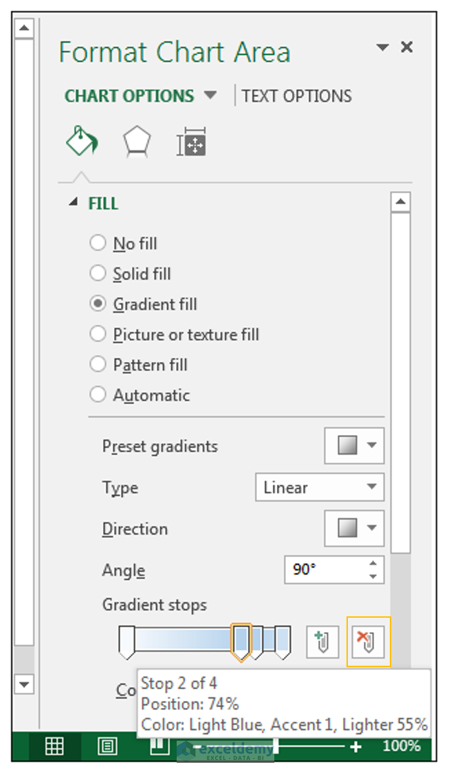
Format Chart Axis in Excel - Axis Options However, In this blog, we will be working with Axis options, Tick marks, Labels, Number > Axis options> Axis options> Format Axis Pane. Axis Options: Axis Options There are multiple options So we will perform one by one. Changing Maximum and Minimum Bounds The first option is to adjust the maximum and minimum bounds for the axis. How to make a quadrant chart using Excel - Basic Excel Tutorial To create it, follow these steps 1. Click on an empty cell 2. Go to the Insert tab 3. On the Charts dialog box, select the X Y (Scatter) to display all types of charts. 5. Click Scatter. An empty chart will appear on your worksheet. Add values to the chart. 1. Right-click on the empty chart area and choose 'Select Data.' 2. How to Add Labels to Scatterplot Points in Excel - Statology Step 3: Add Labels to Points. Next, click anywhere on the chart until a green plus (+) sign appears in the top right corner. Then click Data Labels, then click More Options…. In the Format Data Labels window that appears on the right of the screen, uncheck the box next to Y Value and check the box next to Value From Cells. How to plot a ternary diagram in Excel - Chemostratigraphy.com It may be useful to display the actual ternary values next to the data points in the diagram. If you (right mouse click on data points > Add Data Labels), Excel will display by default the Y-Value, i.e., the values from column L. Double-click in the data labels and you can add the X-Value and number of digits to be displayed. This may be ...
Point.DataLabel property (Excel) | Microsoft Docs This example turns on the data label for point seven in series three on Chart1, and then it sets the data label color to blue. VB With Charts ("Chart1").SeriesCollection (3).Points (7) .HasDataLabel = True .ApplyDataLabels type:=xlValue .DataLabel.Font.ColorIndex = 5 End With Support and feedback PDF not displaying graph markers/data points when exporting from excel Copied. Have been using excel to PDF to generate reports for the longest time via the >file >save as > PDF. Somewhere over the past week my graph data points fail to display on the report. See image below. Its a requirement that i have these data points on the report. If i go file > print > microsoft print to PDF it includes these points. Excel - adding new data points to an existing chart - Microsoft Tech ... When I right-click on one of the three series shown in my chart and then choosing "select data" the Select Data Source window which appears states that "the data range is too complex to be displayed". I would be most grateful if anyone could advise the next steps to take to display on my chart the additional data I have added to my table. Labels: Using VBA to Loop Through and Automatically Position Data Labels? With mychart.Chart.SeriesCollection (1) Dim myvalues myvalues = .Values Dim i As Long For i = LBound (myvalues) To UBound (myvalues) If .Points (i).HasDataLabel And myvalues (i) < 0 And myvalues (i) > -40 Then Selection.Position = xlLabelPositionOutsideEnd Selection.Top = 146.623 Else Selection.Position = xlLabelPositionOutsideEnd End If Next
How To Make a Chart In Excel | Deskbright
excel - Formatting Data Labels on a Chart - Stack Overflow Macro to select last data point in line chart and add a data label. 1. Excel XY chart coordinates for data labels loop through multiple chart template. 0. Loop through chart and altering labels (Category Name) 0. PivotChart Data Labels from Range in VBA. 2.
Excel Dashboard Templates Fixing Your Excel Chart When the Multi-Level Category Label Option is ...
How to Add Leader Lines in Excel? - GeeksforGeeks Leader Lines are the lines that connect data labels and data points in a chart. Before excel 2013 leader lines were available only for pie charts but after excel 2013 update leader lines could be built for any type of chart. Leader lines make complex charts more understandable. Below is a pie chart format is shown,
Format Number Options for Chart Data Labels in Excel 2011 for Mac
Custom Chart Data Labels In Excel With Formulas Select the chart label you want to change. In the formula-bar hit = (equals), select the cell reference containing your chart label's data. In this case, the first label is in cell E2. Finally, repeat for all your chart laebls. If you are looking for a way to add custom data labels on your Excel chart, then this blog post is perfect for you.

35 How To Label Data Points In Excel - Labels For You
support.microsoft.com › en-us › officeAdd or remove data labels in a chart - support.microsoft.com Add data labels to a chart Click the data series or chart. To label one data point, after clicking the series, click that data point. In the upper right corner, next to the chart, click Add Chart Element > Data Labels. To change the location, click the arrow, and choose an option. If you want to ...
How to Add Data Labels in Excel - Excelchat | Excelchat
How can I get data labels to show for each column in a bar chart? Turn on 'Overflow text' under Data label' Format tab. Also, you can adjust the position of the Data Label by switching to 'Outside End' or 'Inside Center' so that your Data Label gets displayed properly. If this post helps, then mark it as 'Accept as Solution ' so that it could help others. Regards, Sanket Bhagwat View solution in original post

Excel: How to make an Excel-lent bull's-eye chart
How to Add Axis Titles in a Microsoft Excel Chart Click the Add Chart Element drop-down arrow and move your cursor to Axis Titles. In the pop-out menu, select "Primary Horizontal," "Primary Vertical," or both. If you're using Excel on Windows, you can also use the Chart Elements icon on the right of the chart. Check the box for Axis Titles, click the arrow to the right, then check ...
How to Make a Pie Chart in Excel & Add Rich Data Labels to The Chart!
How to: Display and Format Data Labels - DevExpress After you create a chart, you can add a data label to each data point in the chart to identify its actual value. By default, data labels are linked to data that the chart uses. When data changes, information in the data labels is updated automatically. If required, you can also display custom information in a label.

Excel 2010 pie chart data labels in case of "Best Fit"
How to add a single vertical bar to a Microsoft Excel line chart In the Chart Layouts group, click Add Chart Element. From the dropdown, choose Axes. From the resulting submenu, choose Secondary Vertical ( Figure J ), which displays the axes values to the right...
Excel Dashboard Templates Create Dynamic Excel Chart Conditional Labels and Callouts
Chart.ApplyDataLabels method (Excel) | Microsoft Docs expression. ApplyDataLabels ( Type, LegendKey, AutoText, HasLeaderLines, ShowSeriesName, ShowCategoryName, ShowValue, ShowPercentage, ShowBubbleSize, Separator) expression A variable that represents a Chart object. Parameters Example This example applies category labels to series one on Chart1. VB Copy Charts ("Chart1").SeriesCollection (1).

Improve your X Y Scatter Chart with custom data labels
How to Create a Line Chart in Microsoft Excel Select the data you want to display in the chart and go to the Insert tab. Click the Insert Line or Area Chart drop-down arrow. Choose the type of line chart you want to use. On Windows, you can...
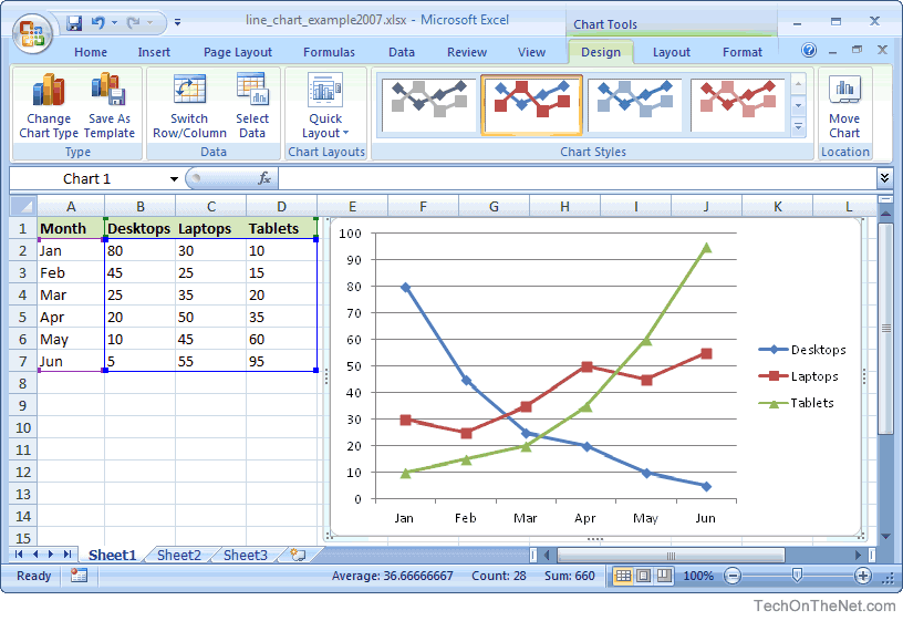
MS Excel 2007: How to Create a Line Chart
How can I format individual data points in Google Sheets charts? The trick is to create annotation columns in the dataset that only contain the data labels we want, and then get the chart tool to plot these on our chart. Add annotations in new columns next to the datapoint you want to add it to, and the chart tool will do the rest. So if you set up your dataset like this:

How to create pie of pie or bar of pie chart in Excel?
How to add legend title in Excel chart - Data Cornering Go to the Insert tab, and on the right side will be a text box. Selec and draw it over the place where you want it in the chart. If you want the text in the same formatting as in the legend, try format painter. Select legend, click on format painter, and then on the text box. As a result, here is my Excel chart with added legend title.

How to Make Charts and Graphs in Excel | Smartsheet
› documents › excelHow to add or move data labels in Excel chart? - ExtendOffice To add or move data labels in a chart, you can do as below steps: In Excel 2013 or 2016. 1. Click the chart to show the Chart Elements button . 2. Then click the Chart Elements, and check Data Labels, then you can click the arrow to choose an option about the data labels in the sub menu. See screenshot:
How-to Add Custom Labels that Dynamically Change in Excel Charts - Excel Dashboard Templates
Excel Waterfall Chart: How to Create One That Doesn't Suck Click inside the data table, go to " Insert " tab and click " Insert Waterfall Chart " and then click on the chart. Voila: OK, technically this is a waterfall chart, but it's not exactly what we hoped for. In the legend we see Excel 2016 has 3 types of columns in a waterfall chart: Increase. Decrease.
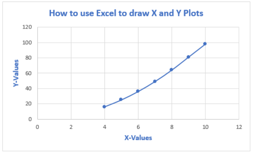
How To Plot X Vs Y Data Points In Excel | Excelchat
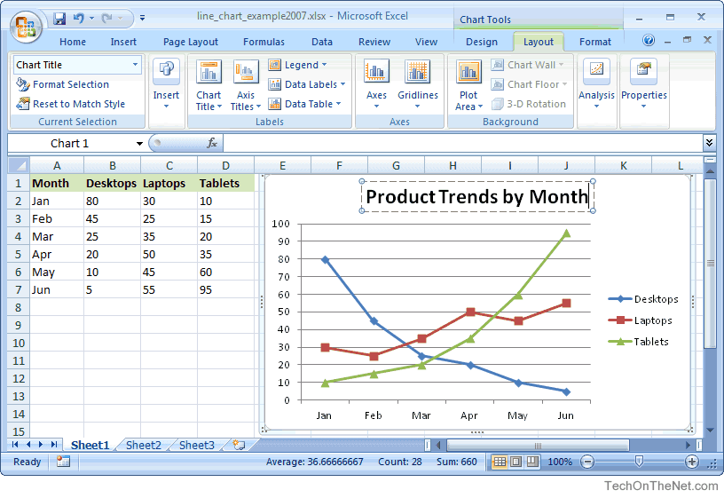
MS Excel 2007: How to Create a Line Chart

How to create chart across/from multiple worksheets in Excel?
Post a Comment for "41 excel chart add labels to data points"