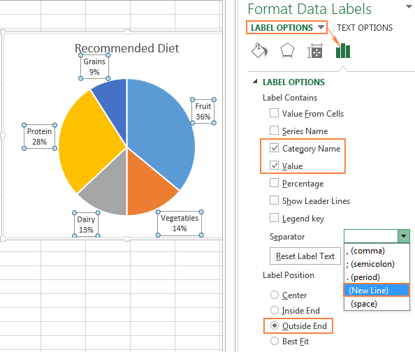
45 use the format data labels task pane to display category name and percentage data labels

Exp19_Excel_AppCapstone_Intro_Collection Project - Chegg Add data labels for categories and percentages; remove value data labels. Change the font size to 16 pt. bold, and Black, Text 1 font color for the data labels Explode the Masterwork Anniversary Edition slice by 15% and change the full color to Light Blue Hint: Use the Format Data Point task pane. Solved step by step instruction 2 A pie chart is an | Chegg.com Use the Insert tab to create a pie chart from the Question: step by step instruction 2 A pie chart is an effective way to visually illustrate the percentage of the class that earned A, B, C, D, and F grades. Use the Insert tab to create a pie chart from the This problem has been solved! See the answer step by step instruction Expert Answer

How to show percentages on three different charts in Excel To convert the calculated decimal values to percentages, right-click on the selected cells and click Format Cells. Alternatively, press CTRL+1 on the keyboard to open the Format Cells dialogue box. 3. In the Format Cells dialogue box, make sure that the Number tab is selected and in the Category list select Percentage.

Use the format data labels task pane to display category name and percentage data labels

Format Chart Axis in Excel - Axis Options Analyzing Format Axis Pane. Right-click on the Vertical Axis of this chart and select the "Format Axis" option from the shortcut menu. This will open up the format axis pane at the right of your excel interface. Thereafter, Axis options and Text options are the two sub panes of the format axis pane. How to: Display and Format Data Labels - DevExpress In particular, set the DataLabelBase.ShowCategoryName and DataLabelBase.ShowPercent properties to true to display the category name and percentage value in a data label at the same time. To separate these items, assign a new line character to the DataLabelBase.Separator property, so the percentage value will be automatically wrapped to a new line. Add a Data Callout Label to Charts in Excel 2013 - Software Tips and Tricks How to Add a Data Callout Label. Click on the data series or chart. In the upper right corner, next to your chart, click the Chart Elements button (plus sign), and then click Data Labels. A right pointing arrow will appear, click on this arrow to view the submenu. Select Data Callout.

Use the format data labels task pane to display category name and percentage data labels. Format Data Labels in Excel- Instructions - TeachUcomp, Inc. To format data labels in Excel, choose the set of data labels to format. To do this, click the "Format" tab within the "Chart Tools" contextual tab in the Ribbon. Then select the data labels to format from the "Chart Elements" drop-down in the "Current Selection" button group. 4.2 Formatting Charts - Beginning Excel, First Edition On the Design tab select the Add Chart Element button, then Data Labels, then Outside End (see Figure 4.36.) Click on one of the Data Labels. Note that all of the data labels for that data series are selected. Using the Home ribbon, change the font to Arial, Bold, size 9. Click on one of the data labels for the other data series. cs 385 exam 3 Flashcards - Quizlet data tab, subtotal, click at each change in: select area, unselect replace current subtotals, click ok Collapse the table to show the grand totals only. click 1 at top left corner Expand the table to show the grand and discipline totals. click 2 at top left corner Use the Auto Outline feature to group the columns. Excel 3-D Pie charts - Microsoft Excel 2016 - OfficeToolTips If you want to create a pie chart that shows your company (in this example - Company A) in the greatest positive light: Do the following: 1. Select the data range (in this example, B5:C10 ). 2. On the Insert tab, in the Charts group, choose the Pie button: Choose 3-D Pie. 3. Right-click in the chart area, then select Add Data Labels and click ...

How to show data label in "percentage" instead of - Microsoft Community Select Format Data Labels Select Number in the left column Select Percentage in the popup options In the Format code field set the number of decimal places required and click Add. (Or if the table data in in percentage format then you can select Link to source.) Click OK Regards, OssieMac Report abuse 8 people found this reply helpful · UsetheFormatDataLabelstaskpanetodisplay - Course Hero Apply 18 point size to the data labels. a. Click green plus data labels center click green plus double click in chart label contains click percentage click values check box click close click home font 18 9. Open the Format Chart Area task pane. Apply the Blue tissue paper texture fill to the chart area of the pie chart. Keep the task pane open. Formatting Data Labels - BusinessView Migration Select from this drop-down menu of preset formats that can be applied to labels. Custom Format. Select this option to use a custom format. See the following table. Style Labels. Click this button to open the Style dialog box, where you can style text. The Format Labels drop-down menu provides a list of preset formats that you can apply to labels. Add or remove data labels in a chart - support.microsoft.com Right-click the data series or data label to display more data for, and then click Format Data Labels. Click Label Options and under Label Contains, select the Values From Cells checkbox. When the Data Label Range dialog box appears, go back to the spreadsheet and select the range for which you want the cell values to display as data labels.

A data label is descriptive text that shows that exact value or name of ... To format the data labels - Double click a data label to open the Format Data Labels task pane. Click the Label Options Icon. Click Label Options to customize the labels, and complete any of the following steps: Select the Label Contains options. The default is Value, but you might want to display additional label contents, such as Category Name. Display the percentage data labels on the active chart. - YouTube Display the percentage data labels on the active chart.Want more? Then download our TEST4U demo from TEST4U provides an innovat... Change the format of data labels in a chart To get there, after adding your data labels, select the data label to format, and then click Chart Elements > Data Labels > More Options. To go to the appropriate area, click one of the four icons ( Fill & Line, Effects, Size & Properties ( Layout & Properties in Outlook or Word), or Label Options) shown here. How do you format data series in Excel? - FAQ-ALL On the Ribbon, select the Chart Tools Format tab, then click Format Selection. The second way: On a chart, select an element. Right-click, then select Format where is the axis, series, legend, title, or area that was selected. Once open, the Formatting Task pane remains available until you close it.

Hướng dẫn xây dựng biểu đồ hình tròn trong Excel, nhiều kỹ thuật hay và hữu ích.

Excel tutorial: How to use data labels When first enabled, data labels will show only values, but the Label Options area in the format task pane offers many other settings. You can set data labels to show the category name, the series name, and even values from cells. In this case for example, I can display comments from column E using the "value from cells" option.

Share :