41 pie chart excel labels

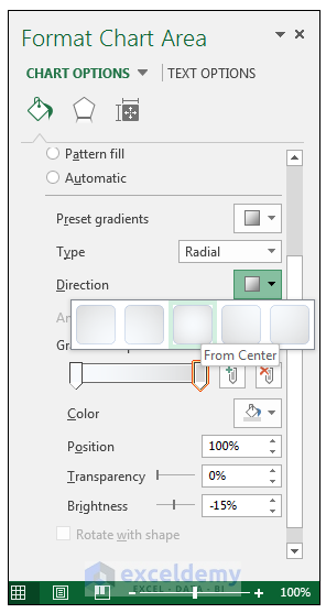
Pie Chart in Excel - Inserting, Formatting, Filters, Data Labels Dec 29, 2021 · Right click on the Data Labels on the chart. Click on Format Data Labels option. Consequently, this will open up the Format Data Labels pane on the right of the excel worksheet. Mark the Category Name, Percentage and Legend Key. Also mark the labels position at Outside End. This is how the chark looks. Formatting the Chart Background, Chart Styles Add or remove data labels in a chart - support.microsoft.com Click the data series or chart. To label one data point, after clicking the series, click that data point. In the upper right corner, next to the chart, click Add Chart Element > Data Labels. To change the location, click the arrow, and choose an option. If you want to show your data label inside a text bubble shape, click Data Callout.

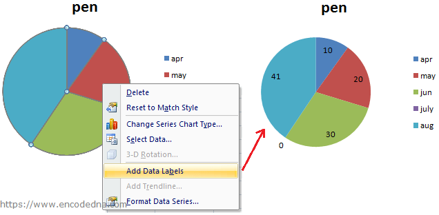
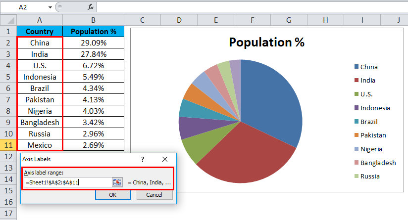
How to show percentage in pie chart in Excel? - ExtendOffice Select the data you will create a pie chart based on, click Insert > I nsert Pie or Doughnut Chart > Pie. See screenshot: 2. Then a pie chart is created. Right click the pie chart and select Add Data Labels from the context menu. 3. Now the corresponding values are displayed in the pie slices.

Pie chart excel labels

Pie of Pie Chart in Excel - Inserting, Customizing, Formatting To insert a Pie of Pie chart:- Select the data range A1:B7. Enter in the Insert Tab. Select the Pie button, in the charts group. Select Pie of Pie chart in the 2D chart section. Adding Data Labels to Pie of Pie Chart The chart inserted in the above section is:- Pie of Pie Chart | Exceljet - Work faster in Excel The Pie of Pie Chart is a built-in chart type in Excel. Pie charts are meant to express a "part to whole" relationship, where all pieces together represent 100%. Pie charts work best to display data with a small number of categories (2-5). The Pie of Pie Chart provides a way to add additional categories to a pie chart without generating a pie chart too complex to read. Edit titles or data labels in a chart - support.microsoft.com On a chart, click the label that you want to link to a corresponding worksheet cell. On the worksheet, click in the formula bar, and then type an equal sign (=). Select the worksheet cell that contains the data or text that you want to display in your chart. You can also type the reference to the worksheet cell in the formula bar.

Pie chart excel labels. How to Rotate Pie Chart in Excel? - WallStreetMojo Move the cursor to the chart area to select the pie chart. Step 5: Click on the Pie chart and select the 3D chart, as shown in the figure, and develop a 3D pie chart. Step 6: In the next step, change the title of the chart and add data labels to it. Then, the chart will look like as Step 7: To rotate the pie chart, click on the chart area. Excel 3-D Pie charts - Microsoft Excel 2016 - OfficeToolTips If you want to create a pie chart that shows your company (in this example - Company A) in the greatest positive light: Do the following: 1. Select the data range (in this example, B5:C10 ). 2. On the Insert tab, in the Charts group, choose the Pie button: Choose 3-D Pie. 3. Right-click in the chart area, then select Add Data Labels and click ... Types of Pie Charts in Excel with Examples - EDUCBA 1. 2D Chart. Click on the Insert option that available on the top, as shown in the below image. Go to the charts segment and select the drop-down of Pie chart, which will show different types of PIE charts available in excel. So, we have 3 different charts under the 2D pie and one under the 3D pie and one under Doughnut. How to Create Bar of Pie Chart in Excel? Step-by-Step To add and format data labels to portions in your Bar of pie chart, follow the steps below: Click anywhere on the blank area of the chart. You will see three icons appear to the right side of the chart, as shown below: Click on the plus icon ('+') , which represents the Chart Elements settings. Check the box next to ' Data Labels '.

How to Create and Format a Pie Chart in Excel - Lifewire Jan 23, 2021 · Select the plot area of the pie chart. Right-click the chart. Select Add Data Labels . Select Add Data Labels. In this example, the sales for each cookie is added to the slices of the pie chart. Change Colors When a chart is created in Excel, or whenever an existing chart is selected, two additional tabs are added to the ribbon. How to Create Pie Charts in Excel (In Easy Steps) 1. Select the range A1:D2. 2. On the Insert tab, in the Charts group, click the Pie symbol. 3. Click Pie. Result: 4. Click on the pie to select the whole pie. Click on a slice to drag it away from the center. Result: Note: only if you have numeric labels, empty cell A1 before you create the pie chart. How to Insert Axis Labels In An Excel Chart | Excelchat We will go to Chart Design and select Add Chart Element Figure 6 - Insert axis labels in Excel In the drop-down menu, we will click on Axis Titles, and subsequently, select Primary vertical Figure 7 - Edit vertical axis labels in Excel Now, we can enter the name we want for the primary vertical axis label. Inserting Data Label in the Color Legend of a pie chart Inserting Data Label in the Color Legend of a pie chart. Hi, I am trying to insert data labels (percentages) as part of the side colored legend, rather than on the pie chart itself, as displayed on the image below. Does Excel offer that option and if so, how can i go about it?

Pie Chart in Excel | How to Create Pie Chart - EDUCBA Step 1: Select the data to go to Insert, click on PIE, and select 3-D pie chart. Step 2: Now, it instantly creates the 3-D pie chart for you. Step 3: Right-click on the pie and select Add Data Labels. This will add all the values we are showing on the slices of the pie. Is there a way to change the order of Data Labels? Replied on April 4, 2018. Hi Keith, I got your meaning. Please try to double click the the part of the label value, and choose the one you want to show to change the order. Thanks, Rena. -----------------------. * Beware of scammers posting fake support numbers here. * Once complete conversation about this topic, kindly Mark and Vote any ... Pie Chart - legend missing one category (edited to include spreadsheet ... Excel is getting confused by your merged cells. If possible, unmerge the cells, and link the label to a single cell. If you don't want to unmerge, then change the label refs in the series formula for the chart. Click on the pie chart, and in the formula bar, change the merged cell refs to a single cell ref: -- instead of: $O$21:$S$21 put $O$21 Pie Chart In Excel | Microsoft Excel Tips | Excel Tutorial | Free Excel ... You have already learned how to create a chart in Excel. A pie chart is created the same way as any other type. Action starts with the selection of data. First prepare a table with data. Then go to the Insert tab in the ribbon Excel. Find and select the Charts section -> Pie. You will insert a pie chart. The question is which one to choose. Pie ...

How to Setup a Pie Chart with no Overlapping Labels | Telerik Reporting

How to Make a Pie Chart in Excel & Add Rich Data Labels to ... A tennis coach at a hypothetical tennis clinic is evaluating the post-game performance of his top-seeded player. He wants to visually present the main types of errors the player made along with the unforced errors. Here we will combine this two errors in a pie chart. So let`s start the procedure. The source data is shown below:

33 How To Label Pie Chart In Excel - Labels Design Ideas 2020

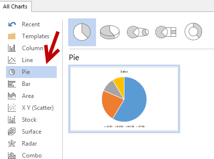
Everything You Need to Know About Pie Chart in Excel How to Make a Pie Chart in Excel Start with selecting your data in Excel. If you include data labels in your selection, Excel will automatically assign them to each column and generate the chart. Go to the INSERT tab in the Ribbon and click on the Pie Chart icon to see the pie chart types. Click on the desired chart to insert.

How to Make a Pie Chart in Excel – Contextures Blog

Making a Pie Chart in Excel - Brigham Young University-Idaho Step 2: Highlight the data. Highlight the data. If you want to have the labels on the chart, you need to highlight the labels of the data as well. Step 3: In Excel, go to INSERT in the menu. Then select CHART. Then select PIE. Excel will automatically create a pie chart for you. You can adjust the size by pushing and pulling on the sides of the ...

How to Create a Pie Chart in Excel using Worksheet Data

How to display leader lines in pie chart in Excel? - ExtendOffice To display leader lines in pie chart, you just need to check an option then drag the labels out. 1. Click at the chart, and right click to select Format Data Labels from context menu. 2. In the popping Format Data Labels dialog/pane, check Show Leader Lines in the Label Options section. See screenshot: 3.

How to Make a Pie Chart in Excel & Add Rich Data Labels to The Chart!

How to Edit Pie Chart in Excel (All Possible Modifications) 9. Change Pie Chart's Legend Position. Just like the chart title and data labels, you can also edit a pie chart in Excel by changing the position of the legend. Follow the simple steps below to do this. 👇. Steps: Firstly, click on the chart area. Following, click on the Chart Elements icon.

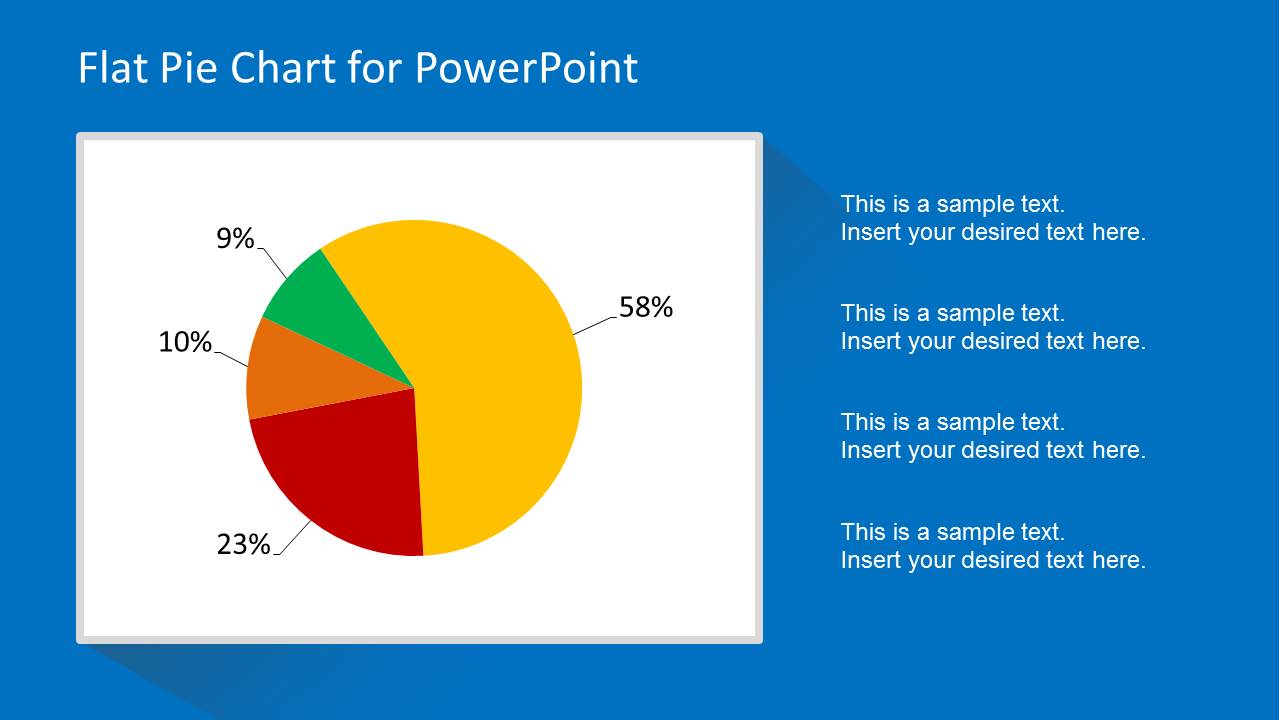
Flat Pie Chart Template for PowerPoint - SlideModel

Display data point labels outside a pie chart in a paginated report ... To prevent overlapping labels displayed outside a pie chart. Create a pie chart with external labels. On the design surface, right-click outside the pie chart but inside the chart borders and select Chart Area Properties.The Chart AreaProperties dialog box appears. On the 3D Options tab, select Enable 3D. If you want the chart to have more room ...

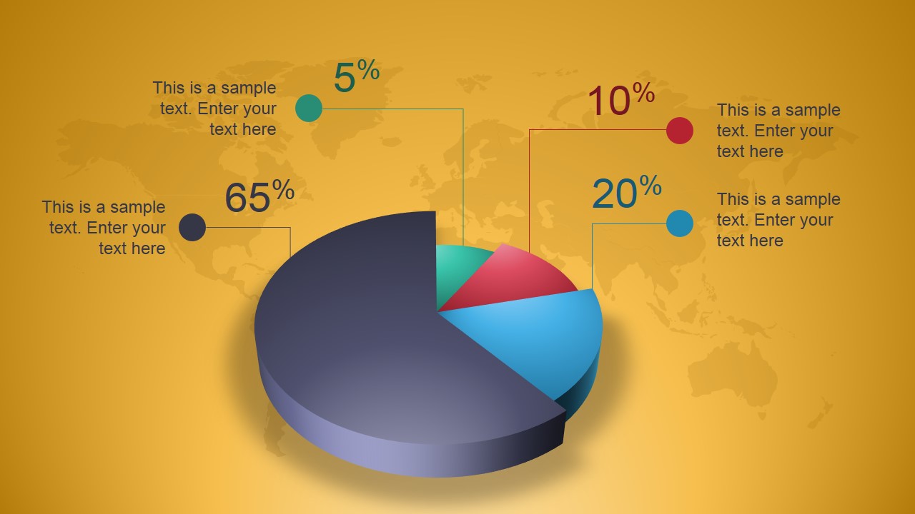
Creative 3D Perspective Pie Chart for PowerPoint - SlideModel

How to Make a PIE Chart in Excel (Easy Step-by-Step Guide) Here are the steps to format the data label from the Design tab: Select the chart. This will make the Design tab available in the ribbon. In the Design tab, click on the Add Chart Element (it's in the Chart Layouts group). Hover the cursor on the Data Labels option.

Pie Chart

How to Make a Pie Chart in Excel (Only Guide You Need) # Formatting Data Labels of the Pie Chart To do this select the More Options from Data labels under the Chart Elements or by selecting the chart right click on to the mouse button and select Format Data Labels. This will open up the Format Data Label option on the right side of your worksheet. Click on the percentage.

how to label pie chart in excel - Labels 2021

How to Create a Pie Chart in Excel | Smartsheet To create a pie chart in Excel 2016, add your data set to a worksheet and highlight it. Then click the Insert tab, and click the dropdown menu next to the image of a pie chart. Select the chart type you want to use and the chosen chart will appear on the worksheet with the data you selected.

How to show percentage in pie chart in Excel?

How to Make a Pie Chart in Excel: 10 Steps (with Pictures) It's at the top of the Excel window, just right of the Home tab. 3 Click the "Pie Chart" icon. This is a circular button in the "Charts" group of options, which is below and to the right of the Insert tab. You'll see several options appear in a drop-down menu: 2-D Pie - Create a simple pie chart that displays color-coded sections of your data.

Do My Excel Blog: How to hide the zero percent labels in an Excel pie chart

Edit titles or data labels in a chart - support.microsoft.com On a chart, click the label that you want to link to a corresponding worksheet cell. On the worksheet, click in the formula bar, and then type an equal sign (=). Select the worksheet cell that contains the data or text that you want to display in your chart. You can also type the reference to the worksheet cell in the formula bar.

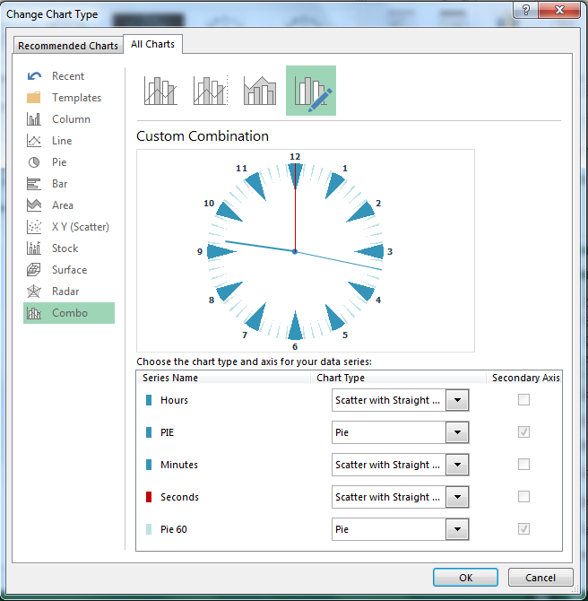
Building an Excel Clock Chart - Xcelanz

Pie of Pie Chart | Exceljet - Work faster in Excel The Pie of Pie Chart is a built-in chart type in Excel. Pie charts are meant to express a "part to whole" relationship, where all pieces together represent 100%. Pie charts work best to display data with a small number of categories (2-5). The Pie of Pie Chart provides a way to add additional categories to a pie chart without generating a pie chart too complex to read.